Bias and Variance

Introduction:

In the vast landscape of machine learning, one of the most crucial challenges we encounter is striking the delicate balance between bias and variance. These twin adversaries can significantly impact the performance of our models, determining their ability to make accurate predictions on unseen data. In this article, we embark on a journey to unravel the intricacies of bias and variance in machine learning, exploring their implications, tradeoffs, and strategies for achieving optimal model performance.

Understanding Bias and Variance:

• What is Bias?

Bias refers to the discrepancy or error between a model’s predicted value and the actual value, stemming from the model’s limitations. These disparities, labeled as bias error or error due to bias, arise when the model’s predictions deviate from the expected outcomes. Bias represents a systematic error in the machine learning process, often originating from incorrect assumptions.

Bias = E[f(x)] – f(x) Where:

E[f(x)] is the expected value of the predictions made by the model across

 multiple training datasets.

f(x) is the true function that we are trying to approximate or predict.

• Low Bias: A low bias value indicates that the model makes fewer assumptions when constructing the target function. Consequently, the model closely aligns with the training dataset.
• High Bias: Conversely, a high bias value signifies that the model relies on numerous assumptions when constructing the target function. Consequently, the model does not closely match the training dataset.

• What is variance?
• Variance refers to the extent of dispersion in data relative to its mean position. In the context of machine learning, variance represents the degree to which the performance of a predictive model varies when trained on different subsets of the training data. Put simply, variance measures the model’s sensitivity to changes in the training dataset, gauging its ability to adapt to new subsets effectively.

Variance = E[(f(x) – E[f(x)])^2]

Where:

E[f(x)] is the expected value of the predictions made by the model across multiple training datasets.

f(x) is the prediction made by the model for input x.

• Low Variance: When a model exhibits low variance, it signifies that the model is relatively stable and less prone to changes in the training data. It can consistently provide reliable estimates of the target function across different subsets of data from the same distribution. However, this scenario often leads to underfitting, where the model fails to capture the underlying patterns in the data and thus struggles to generalize well to both training and test datasets.

• High Variance: On the other hand, high variance indicates that the model is highly sensitive to variations in the training data. This sensitivity results in significant fluctuations in the estimated target function when the model is trained on different subsets of data from the same distribution. While the model may perform exceptionally well on the training data, it often struggles to generalize effectively to new, unseen test data. This phenomenon, known as overfitting, occurs when the model fits the training data too closely, resulting in poor performance on new datasets.

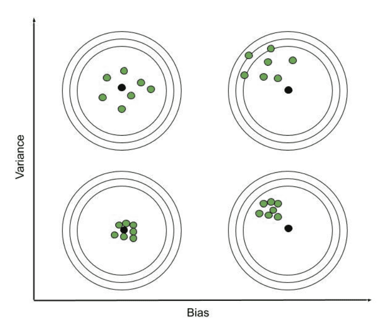
Here is a simple example to understand bias and variance

Imagine you’re trying to predict housing prices based on various features such as location, size, and amenities. Bias represents the error introduced by simplifying the relationship between these features and the price—a model with high bias might assume that all houses have the same value per square foot, regardless of location or other factors. On the other hand, variance measures the model’s sensitivity to small fluctuations in the training data. A high variance model might capture noise in the data, such as random fluctuations in prices, leading to overfitting and poor generalization to new data.

The Bias-Variance Trade off:

Finding the right balance between bias and variance is akin to walking a tightrope. Increasing model complexity tends to reduce bias but increase variance, while decreasing complexity leads to the opposite effect. The goal is to find the sweet spot where both bias and variance are minimized, resulting in a model that can accurately capture the underlying patterns in the data without being overly sensitive to noise.

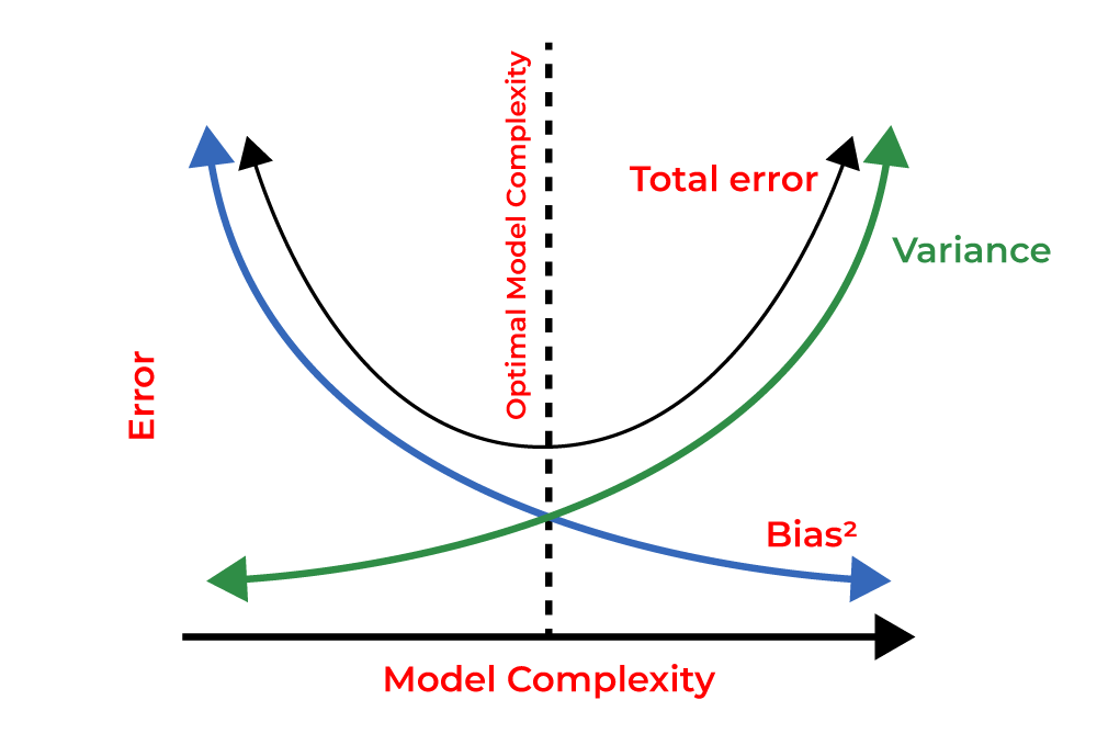
If the algorithm is too simplistic, represented by a linear equation hypothesis, it may exhibit high bias and low variance, rendering it prone to errors. Conversely, overly complex algorithms, characterized by high-degree equation hypotheses, tend to have high variance and low bias, resulting in poor performance on new data entries. Between these extremes lies a pivotal concept known as the Bias-Variance Tradeoff, where the complexity of the algorithm is balanced to mitigate both bias and variance. It’s impossible for an algorithm to simultaneously increase and decrease in complexity. Achieving the ideal tradeoff is akin to finding a delicate equilibrium, illustrated graphically as follows.

Strategies to Address Bias and Variance:

There are several strategies we can employ to tackle bias and variance and achieve the desired balance. To reduce bias, we might consider using more complex models, adding additional features, or fine-tuning model parameters. Conversely, to combat variance, techniques such as regularization, cross-validation, and ensemble learning can be effective. Regularization methods like L1 or L2 regularization help prevent overfitting by penalizing overly complex models, while cross-validation allows us to estimate a model’s performance on unseen data and detect overfitting early on. Ensemble learning, which combines predictions from multiple models, can also help reduce variance and improve robustness.

Model Evaluation and Validation:

Proper model evaluation and validation are critical steps in understanding and managing bias and variance. Metrics such as training error, validation error, and test error provide insights into a model’s performance and help diagnose bias and variance issues. Learning curves and validation curves offer visual aids to guide model selection and fine-tuning decisions, ensuring that our models generalize well to new data.

Real-World Applications and Case Studies:

The impact of bias and variance extends across various domains, from finance and healthcare to marketing and beyond. Real-world case studies illustrate how finding the right balance between bias and variance can lead to significant improvements in model performance. Whether it’s predicting customer churn, detecting fraudulent transactions, or diagnosing medical conditions, mastering bias and variance is essential for building reliable and effective machine learning models.

Conclusion:

In the dynamic landscape of machine learning, navigating the bias-variance balancing act is essential for building models that deliver accurate predictions and actionable insights. By understanding the nuances of bias and variance, and employing appropriate strategies to manage them, we can unlock the full potential of machine learning and drive meaningful impact across diverse domains. As we continue to refine our models and push the boundaries of what’s possible, let us embrace the challenge of achieving the perfect balance between bias and variance, propelling us toward greater success in the exciting world of machine learning.