Understanding Key Performance Metrics for Regression Models

Machine Learning (ML) revolutionizes data analysis by enabling algorithms to learn patterns and make predictions without explicit programming. Regression analysis is at the core of machine learning which is a statistical method crucial for modeling connections between variables and forecasting continuous outcomes. Regression and Machine Learning (ML) combined provide an effective suite of tools for deriving insights from data and enabling well-informed decision-making in a variety of domains.

A number of metrics are essential for measuring the accuracy and reliability of regression models for evaluating their performance. In this article, we focus on such fundamental performance metrics.

Types of Regression Performance Metrics:

• Mean Absolute Error (MAE)
• Mean Squared Error (MSE)
• Root Mean Squared Error (RMSE)
• R-squared (R²) Score

Mean Absolute Error (MAE)

MAE is the most basic performance metric for regression models. The MAE is calculated as the average of the absolute differences between the predicted values and the corresponding actual values. Model accuracy can be easily interpreted using MAE, where lower values represent better performance. However, MAE is vulnerable to data outliers since it does not penalize huge errors more heavily. 

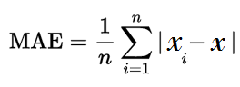
Mathematical Formula: 

Where: 

• n is the number of observations

• x_i is the individual observations
• x is the predicted value

Example:

from sklearn.metrics import mean_absolute_error

y_true = [3, -0.5, 2, 7]

y_pred = [2.5, 0.0, 2, 8]

mae = mean_absolute_error(y_true, y_pred)

print(“Mean Absolute Error (MAE):”, mae)

Output:

Mean Absolute Error (MAE): 0.5

Mean Squared Error (MSE)

MSE is popularly used metric that calculates the average of the squared differences between predicted and actual values. MSE is more sensitive to outliers than MAE since it penalizes greater deviations more severely by squaring the errors. The primary benefit of MSE is that it makes sure all errors are positive, which makes math calculations easier.

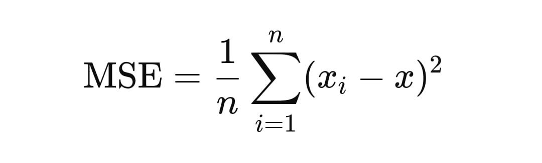
Mathematical Formula: 

Where: 

• n is the number of observations
• x_i is the individual observations
• x is the predicted value

Example:

from sklearn.metrics import mean_squared_error

y_true = [3, -0.5, 2, 7]

y_pred = [2.5, 0.0, 2, 8]

mse = mean_squared_error(y_true, y_pred)

print(“Mean Squared Error:”, mse)

Output:

Mean Squared Error: 0.375

Root Mean Squared Error (RMSE):

The root mean squared error or RMSE is probably the most comprehensible regression model performance metric. Since RMSE is stated in the same units as the dependent variable, comparing it between models is made simpler. Similar to MSE, RMSE provides a fair evaluation of model accuracy by penalizing greater errors more heavily.

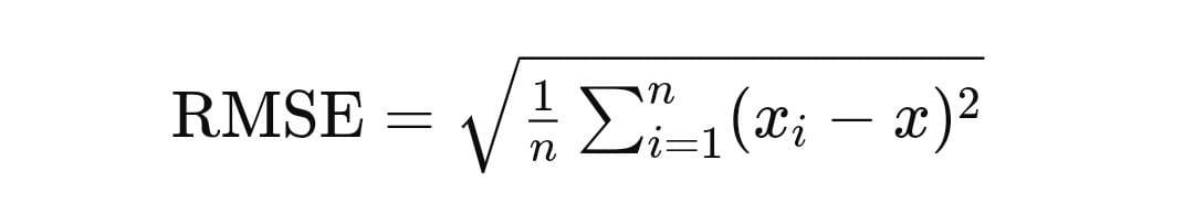
Mathematical Formula: 

Where: 

• n is the number of observations

• x_i is the individual observations
• x is the predicted value

Example:

from sklearn.metrics import mean_squared_error

import numpy as np

y_true = [3, -0.5, 2, 7]

y_pred = [2.5, 0.0, 2, 8]

mse = mean_squared_error(y_true, y_pred)

rmse = np.sqrt(mse)

print(“Root Mean Squared Error:”, rmse)

Output:

Root Mean Squared Error: 0.6123724356957945

R-squared (R²) Score:

R-squared is a popular statistic for evaluating a regression model’s goodness of fit. It shows the percentage of the dependent variable’s variance that the independent factors account for. Higher R-squared values signify a better match; values range from 0 to 1. R-squared, however, can be misleading when applied alone since it ignores overfitting and the existence of irrelevant variables. 

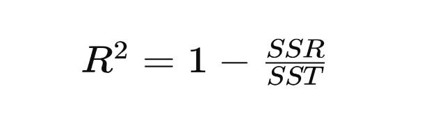
Mathematical Formula: 

Where:

• SSR is the sum of squared residuals (also known as the sum of squared errors), which represents the total variance of the dependent variable that is not explained by the independent variables.
• SST is the total sum of squares, which represents the total variance of the dependent variable.

Example:

from sklearn.metrics import r2_score

y_true = [3, -0.5, 2, 7]

y_pred = [2.5, 0.0, 2, 8]

r2 = r2_score(y_true, y_pred)

print(“R^2 Score:”, r2)

Output:

R^2 Score: 0.9486081370449679

Conclusion:

In conclusion, a number of elements, such as the type of data, the analysis’s goals, and the target audience, must be taken into consideration when choosing the right performance metric for assessing regression models. Even if every statistic provides a different perspective on the performance of the model, it is crucial to carefully weigh the advantages and disadvantages of each. Researchers and practitioners can obtain a thorough grasp of regression model correctness and make wise decisions in their analyses by utilizing a variety of performance metrics.